The Value Factor… Trends

At the start of 2020, the cumulative returns for the classic, Fama-French value factor (HmL) had been zero since 1996, a period of 24 years. After the market crash in March, with value hit especially hard, the period of net zero performance now stretches back to 1994, a couple years after Fama and French first published their three factor model.

That fact raises concerns that value has joined the large group of factors whose outperformance disappeared after publication. However, the returns of value since 1994 do not fit the pattern of a factor that has been arbitraged away. Instead of having flat returns month after month, value has had periods of significant outperformance (1996–97, 2001–07) cancelled out by periods of significant underperformance (1998–2000, 2008–20).

Despite its net zero returns, investors who tilted toward value during the 2001–07 period, for example, would have strongly outperformed the market, provided that they stopped doing so during some of the period since then. Unfortunately, “factor timing” in this manner is anecdotally very difficult.

Strangely, however, that has not been the case since the mid-1990s, as we will see below.

Market Timing

“Timing the market” has the same reputation for difficulty. Yet, there are well-known methods for doing so that have worked well and done so consistently for long periods of time. In particular, you’d have sidestepped the major drawdowns of most bear markets by going to cash whenever the price drops below a long-term moving average, e.g., the 200-day moving average.

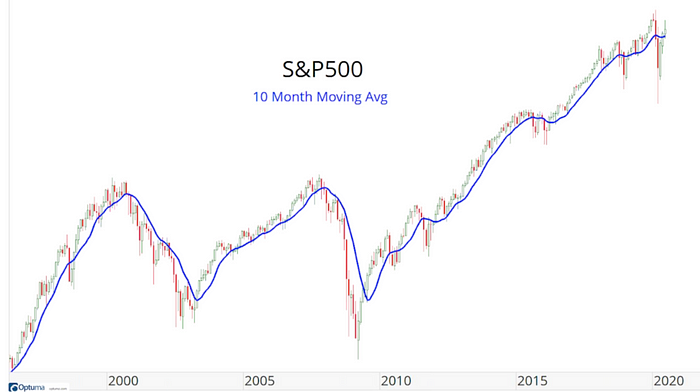
J.C. Parets describes the method shown above as the simplest trend following system he knows. It looks only at monthly closing prices. When price closes above the 10-month moving average, you stay long, and when price closes below the 10-month moving average, you go short (or go to cash).

As the chart shows, this approach would have avoided the major drawdowns of the main bear markets since 1995. Of course, it doesn’t get you out exactly at the top or get you back in exactly at the bottom, but we shouldn’t ask it to do so. As Jesse Livemore wrote,

One of the most helpful things that anybody can learn is to give up trying to catch the last eighth — or the first. These two are the most expensive eighths in the world.

Value Timing

Let’s try out Parets’s method with the value factor. Here is what it looks like:

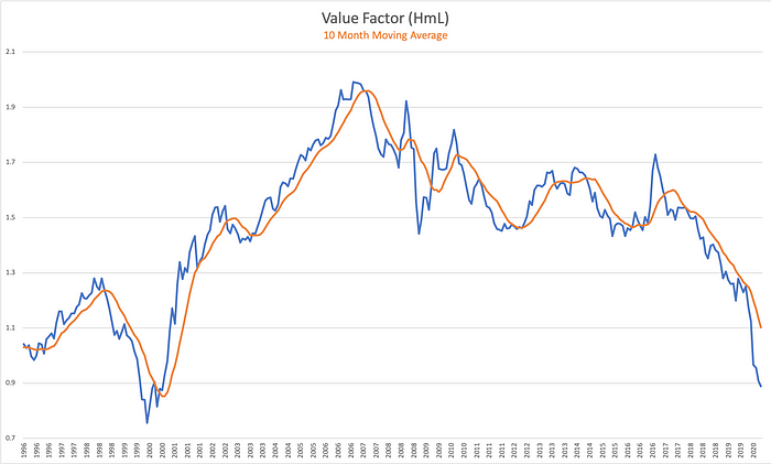
Again, it doesn’t nail every top and bottom, but it gets you on the right side of the major moves. You’d have been long value during most of its outperformance from 2000–07 and short value (long growth) during its most of its underperformance, especially the terrible period 2017–present.

In terms of real returns, while the value portfolio has lost 0.6% per year since 1996, the trend following approach would have gained 6.6% per year. Of course, this is on top of the market returns. Both of these portfolios are market neutral, and adding them onto market returns of 9.0% per year since 1996, would give returns of 8.4% per year for a value-tilted portfolio versus 15.7% per year for the trend-following approach that will be tilted either toward value or toward growth each month.

This strategy could be easily implemented via ETFs. For example, we could use the iShares Russell 1000 Value (IWD) and Growth (IWF) ETFs. Those two have been around since 2000. During that period, each has earned 5–6% per year. However, a trend-following approach that switches between them monthly would have returned 10% per year. (Obviously, this is a better fit with a tax-advantaged account than a taxable one.)

For those who object to owning growth stocks, you can also use trend following for turning a value tilt on and off (without ever tilting toward growth). This is analogous to using trend following on the S&P 500 by going to cash when it closes below its 10-month moving average rather than shorting the market during those periods. Turning off a value tilt when value is in a downtrend would have kept you out of value stocks during most its long periods of underperformance, turning the value factor’s -0.6% annualized returns into 3.3% per year since 1996.

The Current Market

As you can see from the chart above, the value factor (as of June 2020) is in a clear and obvious downtrend at present. While Cliff Asness and others may be correct that this is about to change (and the last two months have given some evidence in this direction), it is still a long way from crossing back over the 10-month moving average.

It will take more than a few good months to retrace the significant drawdown in value over the last four years. My expectation is that, if value is about to recover, it will, as in the past, do so through an extended period of outperformance, which will appear as an uptrend in chart.

My plan, at present, is to follow Livermore’s advice and avoid trying to capture the first eighth of that move. I’m happy to wait until the value portfolio closes above the 10-month moving average before tilting back toward value. In the meantime, that means sleeping a little easier with less exposure extremely risky industries like oil E&P and regional banks.

Looking Forward

It is plain from the chart of the value factor above that it is not behaving like a factor that has been arbitraged away. Such a factor would have a chart that goes mostly flat, with little return, positive or negative, in any month. Instead, value continues to have large swings in both directions.

In particular, despite cumulative returns close to zero since 1996, it has continued to exhibit large trends since that time. Hence, it provides the opportunity to generate alpha through basic trend following strategies, like the one outlined above.

I’ll describe some more advanced approaches, with even more alpha, in a future post.